Memory Management

Introduction

Over time we have known that the performance of the system depends on the main memory, how much is available and how it optimizes when jobs are being processed. Therefore the management of the main memory must be as efficient as possible.

The design on the main memory has grown and we have evolved from the main memory being a unit that we can physically see to something that is abstracted far away inside the internals of a CPU.

We will take a look at some of the attempts made at solving this problem.

1. Single-User Contiguous Allocation

The very first attempt at solving this problem was in a non-multiprogramming environment i.e. only one job can be work on at a given time. When jobs are ready for processing, they are executed sequentially that is it was a First-Come-First-Serve Algorithm.

One visible constraint to this was that the size of memory was small so a job larger than the size of the memory never gets executed.

Algorithm

A simplified (and abstracted) version of the algorithm.

1. Store the first memory location of the program into the base register (for memory protection)
2. Set program counter (it keeps track of memory space used by the program) equal to address of first memory location
3. Read the first instruction of the program
4. Increment program counter by the number of bytes in the instruction
5. Has the last instruction been reached?
     if yes, then stop loading the program
     else, then continue with step 6
6. Is the program counter greater than memory size?
     if yes, then stop loading the program
     else, then continue with step 7
7. Load instruction in memory
8. Read the next instruction of the program
9. Go to step 4

Step 6 handles the scenario whereby a program's size is more than the memory's size.

2. Fixed Partition

This attempt allowed job processing in a multi-programming environment. Partitions are configured at the start-up and remain fixed until the system is rebooted. Partitions also helped to preserve a job's memory space.

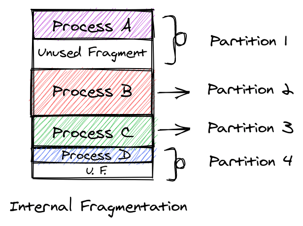
Depending on the type, partitions can be sized equally or varied. In a case where partition sizes are varied, it helps to reduce the occurrence of internal fragmentation.

Internal fragmentation occurs when a job uses less than the space that is allocated to it.

This algorithm is flexible because it allows multiple jobs to run at the same time.

Some of the problems are that

1. If the sizes of the partitions are too small, larger jobs don't get processed or wait until there is a partition large enough to contain them.
2. If the sizes are too large, it increases the rate of internal fragmentation and total turnaround time for a job.
3. Jobs that are larger than the sizes of the partitions but less than the size of the memory never get processed.

Algorithm

1. Get the size of the job.
2. If the size of job > size of the largest partition, reject job
   else go to step 3
3. Set i = 1. // i is the counter.
4. While i <= number of partitions in memory
    if job size > memory partition size(i)
      then i = i + 1
    else
      if memory partition status(i) = ’FREE’
          then load job into memory partition(i)
            change memory partition status(i)  to ’BUSY’
            go to step 1
      else i = i + 1
5. No partition available at this time, put the job in the waiting queue.
6. Go to step 1 to handle the next job.

3. Dynamic Partitions

This method didn't require partitions to be configured at startup but allowed jobs to take as much space as they need and this solved the issue with internal fragmentation.

Jobs can be loaded into memory based on whether they fit into the first partition available i.e. first fit or whether they fit into the partition that leads to the least amount of memory wasted i.e. best fit.

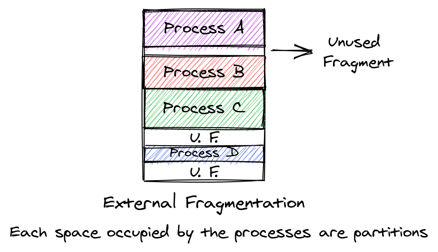
However, this didn't completely solve the issue with memory wastage. External fragmentation started to occur because some jobs began to come in and they couldn't fit into the partitions created by previous jobs.

Memory Deallocation

After a block of memory has been used, there is a need to release the block back to the system and this process is called Memory Deallocation.

In a Fixed Partition system, the status of the block is reset back to FREE but the process is quite different in a Dynamic Partition system.

Three situations may occur when a block of memory is to be freed.

1. The block to be deallocated is adjacent to another free block.
2. The block to be deallocated is between two free blocks.
3. The block to be deallocated is isolated from other free blocks.

Algorithm for Deallocation

if job_location is adjacent to one or more free blocks
  then
  if job_location is between two free blocks
    Then merge all three blocks into one block
    memory_size(counter-1) = memory_size(counter-1) + job_size + memory_size(counter+1)
    set status of memory_size(counter+1) to null entry
  else
    merge both blocks into one
    memory_size(counter-1) = memory_size(counter-1) + job_size
else
  search for null entry in free memory list
  enter job_size and beginning_address in the entry slot
  set its status to “free”

4. Relocatable Dynamic Partitions

To solve the issue of External Fragmentation that occurred in a Dynamic Partition System, Relocatable Dynamic Partitions were created.

The basic idea was that memory spaces that were in use would be relocated into one part of the memory while the free memory is collected into one huge block of memory. This method is referred to as Garbage Collection or Defragmentation.

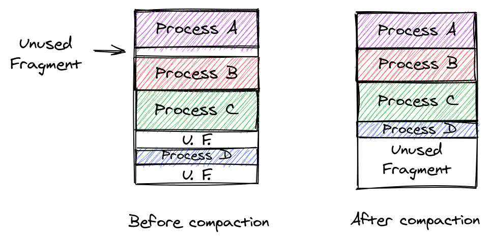
At first, the memory blocks in use would be relocated so that they are contiguous then every memory address and reference to a memory address would need to be updated to reflect their new memory location.

For this process, two registers would be used to make sure that everything is updated correctly. They are the Bounds and Relocation Registers.

The Bounds register is used to store the highest (or lowest) location in memory accessible by each program.

While the Relocation Register contains the value, which could be positive or negative, and that must be added to each address referenced in the program so that the memory addresses are correctly accessed after relocation.

The only drawback to this method is that while the Operating system is compacting the memory no other tasks can be completed and this would add an overhead to the turnaround time of each job.

To reduce the timing of compaction, the operating system has three options. To compact:

1. When the memory is busy.
2. When there are many jobs are waiting.
3. When the waiting time is too long.